Getting Started¶

This tutorial provides explanation for the various modes available for itmlogic.

Firstly a summary of the main primary parameters, secondary parameters and output values is given.

Primary input parameters¶

Parameters	Description
mdp	Controlling
dist	Distance
hg	Antenna structural heights
wn	Wave number
dh	Terrain irregularity
ens	Surface refractivity
gme	Earth’s effective curvature
zgnd	Surface transfer impedance
ze	Effective antenna heights
dl	Horizon distances
the	Horizon elevation angles

Secondary parameters (computed in lrprop)¶

Parameters	Description
dlsa	Line-of-sight distance
dx	Scatter distance
ael, ak1, ak2	Line-of-sight coefficients
aed, emd	Diffraction coefficients
aes, ems	Scatter coefficients
dls	Smooth earth horizon distances
dla	Total horizon distance
tha	Total bending angle

Output values¶

Output values	Description
kwx	Error indicator
aref	Reference attenuation

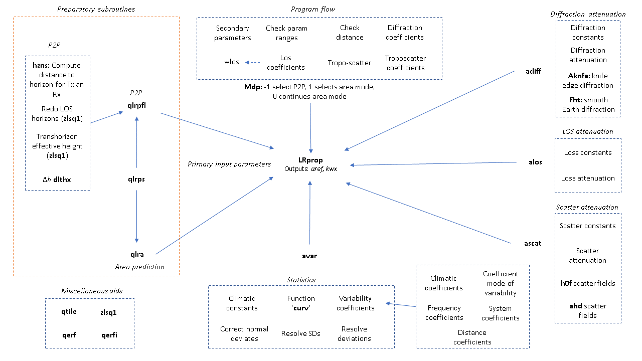
Figure 1 provides an overview of the program flow, subroutines and statistics.

Longley-Rice Irregular Terrain Model Scripts, Routines and Functions¶

The model can run in one of two modes: ‘area prediction mode’ or ‘point-to-point’ prediction mode.

Area Prediction Mode¶

A reproducible example for the Crystal Palace radio transmitter (South London) is provided using a single Digital Elevation Model (DEM) tile. Use the following to run the code:

python scripts/area.py

The repo already includes a DEM tile for London (see the .tif in the data folder).

For simplicity, this example specifies the coordinates of the transmitter as a point feature. This is a standard GeoJSON-like Python dict, as you would get from using shapely to read point features from a file:

transmitter = {
    'type': 'Feature',
    'geometry': {
        'type': 'Point',
        'coordinates': (-0.07491679518573545, 51.42413477117786)
        },
    'properties': {
        'id': 'Crystal Palace radio transmitter'
    }
}

An estimated range (cell_range) is also provided as a maximum cell radius (in meters).

To assess landscape elevation the terrain_area function is imported from the terrain_module. The function enables the estimation of the Terrain Irregularity Parameter (tip), for a cell radius of 20,000 meters (20 km):

tip = terrain_area(dem_path, tx_coordinate_0, tx_coordinate_1, cell_range)

The tip is the inter-decile range for all elevation values (the range between the top 10% and bottom 10% of values). This parameter can then be passed to the itmlogic_area function:

output = itmlogic_area(tip)

As the itmlogic_area is used here to merely demonstrate the code functionality, a user will need to adapt parameters to their specific scenario. For example, the user will want to specify the specific antenna heights, frequency to be modelled and local atmospheric conditions. The main user defined parameters can be set via the main_user_defined_parameters dict, but environmental and statistical paramters will need to be adjusted by the user in the itmlogic_area function.

In the given scenario, the propagation loss across this terrain is estimated for a certain distance, at a specific confidence level, and returned as a list of dicts named output:

output = [
    {
        'distance_km': 10,
        'confidence_level_%': 50,
        'propagation_loss_dB': 111.6920084
    },
    {
        'distance_km': 10,
        'confidence_level_%': 90,
        'propagation_loss_dB': 121.5943795
    },
    ...
]

The results are then written to a csv file in the processed data folder (‘uarea_output.csv).

We also provide an example which spans more than one coverage tile, as defined in:

python scripts/area_2tiles.py

Point-to-Point Mode¶

In contrast to the area prediction mode, the point-to-point mode focuses on a single path across an area of irregular terrain between a transmitter and receiver. To use the reproducible example for p2p, run:

python scripts/p2p.py

The example given is based on the original radio propagation scenario used which is between the Crystal Palace radio transmitter in South London and a receiver in the small village of Mursley in Buckinghamshire, England. For consistency, itmlogic also uses this example, particularly for providing tests for the codebase, to guarantee reliability.

Like the area prediction function, the itmlogic_p2p is used here to merely demonstrate the code functionality, so a user will need to adapt parameters to their specific scenario. For example, the user will want to specify the specific antenna heights, frequency to be modelled and local atmospheric conditions. The main user defined parameters can be set via the main_user_defined_parameters dict, but environmental and statistical paramters will need to be adjusted by the user in the itmlogic_p2p function.

To begin, the transmitter is specified as a point feature:

transmitter = {
    'type': 'Feature',
    'geometry': {
        'type': 'Point',
        'coordinates': (-0.07491679518573545, 51.42413477117786)
        },
    'properties': {
        'id': 'Crystal Palace radio transmitter'
    }
}

Along with the receiver:

receiver = {
    'type': 'Feature',
    'geometry': {
        'type': 'Point',
        'coordinates': (-0.8119433954872186, 51.94972494521946)
        },
    'properties': {
        'id': 'Mursley'
    }
}

The terrain path is then specified as a line feature:

line = {
    'type': 'Feature',
    'geometry': {
        'type': 'LineString',
        'coordinates': [
                (
                    transmitter['geometry']['coordinates'][0],
                    transmitter['geometry']['coordinates'][1]
                ),
                (
                    receiver['geometry']['coordinates'][0],
                    receiver['geometry']['coordinates'][1]
                ),
            ]
        },
    'properties': {
        'id': 'terrain path'
    }
}

Using the terrain_p2p function from the terrain_module we can get the terrain profile, over a set distance, with each point across the terrain profile being returned as a GeoJSON object.

measured_terrain_profile, distance_km, points = terrain_p2p(
    dem_folder, line
)

A list of terrain elevation values (measured_terrain_profile) (in meters) is returned:

measured_terrain_profile = [
    109, 66, 28, 48, 29, 32, 29, 20, 13, 9...
]

These data can then be passed to the itmlogic_p2p function along with the distance (km) of the link:

output = itmlogic_p2p(original_surface_profile_m, distance_km)

The results are returned in a list of dicts called output containing the path loss over the link distance given certain reliability and confidence levels.

output = [
    {
        'distance_km': 77.8,
        'reliability_level_%': 1,
        'confidence_level_%': 50,
        'propagation_loss_dB': 128.5969039310673
    },
    {
        'distance_km': 77.8,
        'reliability_level_%': 1,
        'confidence_level_%': 90,
        'propagation_loss_dB': 137.64279211442656
    },
    ...
]